


Our Product Ranges
Shop
All Products
₹114,000.00₹152,000.00
₹234,000.00₹278,000.00
₹88,000.00₹128,000.00
₹198,000.00₹235,000.00
₹120,000.00₹175,000.00
₹13,500.00₹16,000.00
₹192,000.00₹198,000.00
₹285,000.00₹326,000.00
₹22,000.00

₹26,000.00₹32,000.00
₹835,000.00₹925,000.00
₹199,999.00₹215,000.00
₹357,500.00₹375,000.00
₹38,000.00₹45,000.00
₹38,000.00₹45,000.00
₹110,000.00₹138,000.00
₹110,000.00₹138,000.00
₹2,800.00

₹4,000.00₹5,000.00

₹4,000.00₹5,000.00
₹93,500.00₹125,000.00

₹129,000.00₹155,000.00
Blogs & Events

20 May 2026
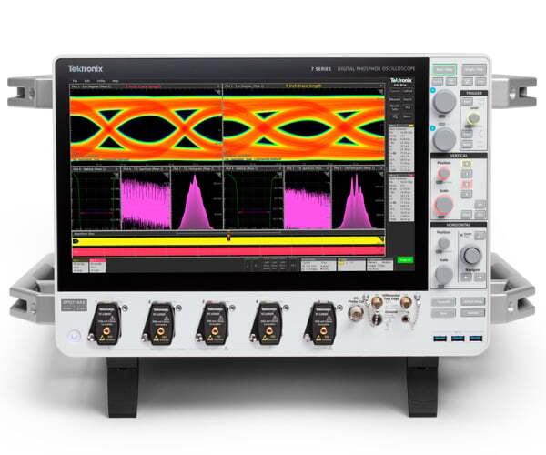
7 Series DPO
Digital Phosphor Oscilloscope
The 7 Series DPO delivers unparalleled signal fidelity, high ENOB, low noise, low jitter, fast measurement throughput ...
20 May 2026
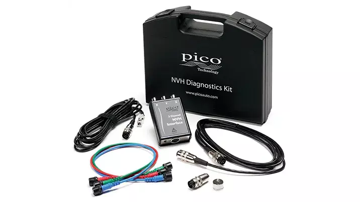
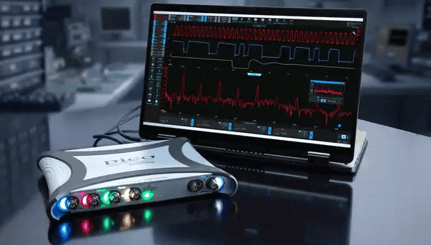
PicoScope
PicoBNC+ NVH Diagnostics System
Three axes into one channel: Greater test flexibility
Auto-probe recognition: Faster, error-free setup ...
01 June 2026
New!
PicoScope 5000E Series
The PicoScope 5000E Series are the first four-channel oscilloscopes to offer 16-bit resolution, Up to 500MHz Bandwidth …